Kaggle Submission for Titanic Dataset
Exploratory Data Analysis and survival prediction with CatBoost algorithm.

Hello, data science enthusiast. In this blog post, I will guide through Kaggle’s submission on the Titanic dataset. We will do EDA on the titanic dataset using some commonly used tools and techniques in python. And then build some Machine Learning models to predict the target features. Want to revise what exactly EDA is? Here is my article on Introduction to EDA.
In one of my initial article Building Linear Regression Models, I explained how to model and predict different linear regression algorithm. In that case, the dataset I used had all features in numerical form. But most of the real-world data set holds lots of non-numerical features. We must transform those non-numerical features into numerical values. The same issue arises in this Titanic dataset that’s why we will do a few data transformation here. Without any further discussion, let’s begin with downloading data first. Here is the link to the Titanic dataset from Kaggle.
Import all the relevant dependencies we need:
You might get some error latter on telling you some libraries you might not have. If so you must install it then. While I was doing this task inspired by Daniel Bourke’s article, I had to install missingo and catboost initially on my jupyter notebook.
#import dependencies
%matplotlib inline#start python imports
import math, time, random, datetime#data manupilation
import numpy as np
import pandas as pd#visualization
import matplotlib.pyplot as plt
import missingno
import seaborn as sns
plt.style.use('seaborn-whitegrid')# preprocessing
from sklearn.preprocessing import OneHotEncoder,LabelEncoder, label_binarize#Machine Learning
import catboost
from sklearn.model_selection import train_test_split
from sklearn import model_selection, tree, preprocessing, metrics, linear_model
from sklearn.svm import LinearSVC
from sklearn.ensemble import GradientBoostingClassifier
from sklearn.neighbors import KNeighborsClassifier
from sklearn.naive_bayes import GaussianNB
from sklearn.linear_model import LinearRegression, LogisticRegression, SGDClassifier
from catboost import CatBoostClassifier, Pool, cv#ignore warnings for now
import warnings
warnings.filterwarnings('ignore')
Loading the data set:
I have saved my downloaded data into file “data”. While downloading, train and test data set are already separated. and there is one more csv file for example for what submission should look like. so let’s load each file with the respective name.
# Import train and test data
train= pd.read_csv('data/train.csv')
test=pd.read_csv('data/test.csv')
gender_submission=pd.read_csv('data/gender_submission.csv') # example of what a submission should look like
View first 15 rows in train dataset.
# view the tranning data
train.head(15)
Let’s view number of passenger in different age group.
train.Age.plot.hist()
View first 5 rows in test dataset.
#view the test data same as train data
test.head()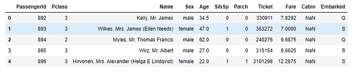
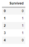
Now first 5 rows of gender_submission data set. This is an example data frame for our final submission data frame.
#view the example submission dataframe
gender_submission.head()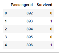
Data Descriptions:
You must have read the data description while downloading the dataset from Kaggle. If not here is what each feature represents.
Survival: 0 = No, 1 = Yes
pclass (Ticket class): 1 = 1st, 2 = 2nd, 3 = 3rd
sex: Sex
Age: Age in years
sibsp: number of siblings/spouses aboard the Titanic
parch: number of parents/children aboard the Titanic
ticket: Ticket number
fare: Passenger fare
cabin: Cabin number
embarked: Port of Embarkation, C = Cherbourg, Q = Queenstown, S = Southampton
I would strongly suggest you go to Kaggle’s website an read the data set description thoroughly. Understanding the data is must before it’s manipulation and analysis.
Now use df.describe( ) to find descriptive statistics for the entire dataset at once.
#data discription
train.describe()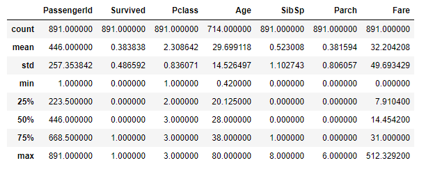
Check missing values:
Before making any analysis lets check if we have any missing values.
# plot graphic of missing values
missingno.matrix(train, figsize=(30,10))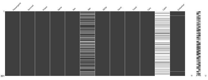
You can clearly see some missing values here. Cabin column has the most missing values. And then Age columns also have quite a few missing values.
It’s important to visualize missing values early so you know where the major holes are in your dataset. And then you can decide which data cleaning and preprocessing are better for filling those holes.
Here is an alternative way of finding missing values.
# alternatively you can see the number of missing values like this
train.isnull().sum()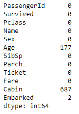
looks like we have few data missing in Embarked field and a lot in Age and Cabin field. We will figure out what would be the best data imputation technique for these features.
To perform our data analysis, let’s create new data frames. We will add the column of features in this data frame as we make those columns applicable for modeling latter on.
df_new =pd.DataFrame()First let’s see what are the different data types of different columns in out train data set.
# different data types in the dataset
train.dtypes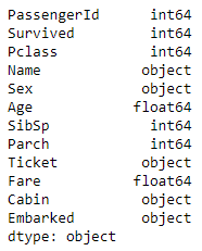
Generally features with a datatype of object could be considered categorical features and those which are floats or ints (numbers) could be considered numerical features. However, as we dig deeper, we might find features that are numerical may actually be categorical.
Explore each of these features individually:
We’ll go through each column iteratively and see which ones are useful for ML modeling latter on. Some columns may need more preprocessing than others to get ready to use an algorithm.
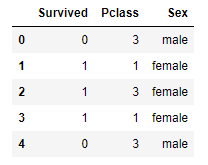
train.head()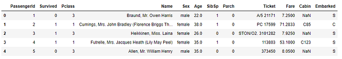
Target Feature: Survived
Description: Whether the passenger survived or not.
Key: 0 = did not survive, 1 = survived
This is the variable we want our machine learning model to predict based on all the others.
# how many people survived?
fig = plt.figure(figsize=(20,1))
sns.countplot(y='Survived', data=train);
print(train.Survived.value_counts())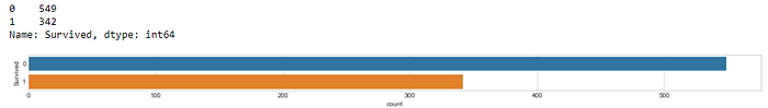
Let’s add this to our new subset dataframe df_new.
df_new['Survived'] = train['Survived']df_new.head()
Feature: Pclass
Description: The ticket class of the passenger.
Key: 1 = 1st, 2 = 2nd, 3 = 3rd
Let’s plot the distribution. We will look at the distribution of each feature first if we can to understand what kind of spread there is across the data set.
# Let's plot the distribution of Pclass
sns.distplot(train.Pclass)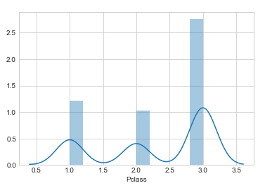
Looks like there is either 1,2 or 3 Pclass for each existing value. This feature column looks numerical but actually, it is categorical. Each value in this feature is Pclass’s type and non of them represent any numerical estimation. Here Pclass 3 has the highest frequency. Now let’s see if this feature has any missing value.
# How many missing variables does Pclass have?
train.Pclass.isnull().sum()
This line of code above returns 0. Since there are no missing values let’s add Pclass to new subset data frame.
df_new['Pclass']= train['Pclass']Feature: Name
Description: The name of the passenger.
First let’s find out how many different names are there?
train.Name.value_counts()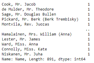
Here length of train.Name.value_counts() is 891 which is same as number of rows. So each row seems to have a unique name. This makes it difficult to find any pattern in Name of a person with survival. Let’s not include this feature Name in the new subset data frame.
Feature: Sex
Let’s view the distribution of gender.
plt.figure(figsize=(20, 5))
sns.countplot(y="Sex", data=train);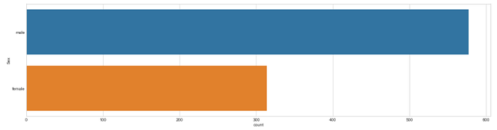
Are there any missing values in the Sex column?
train.Sex.isnull().sum()This line of code above returns 0 . So let’s add this binary variable feature to new subset data frame.
# add Sex to the subset dataframe
df_new['Sex'] = train['Sex']# first five row of df_new
df_new.head()
let’s encode sex varibl with lable encoder to convert this categorical variable to numerical.
df_new['Sex']=LabelEncoder().fit_transform(df_new['Sex'])
df_new.head()
How does the Sex variable look compared to Survival? We can see this because they’re both binarys.
fig = plt.figure(figsize=(8,8))
sns.distplot(df_new.loc[df_new['Survived'] == 1]['Sex'], kde_kws={'bw': 0.1,"label": "Survived"});
sns.distplot(df_new.loc[df_new['Survived'] == 0]['Sex'], kde_kws={'bw': 0.1,"label": "Did not Survived"});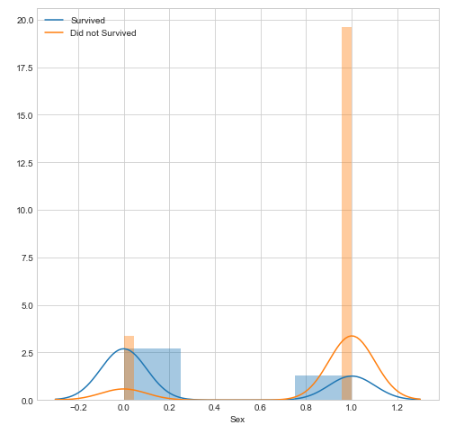
Feature: Age
We already saw that age column has high number of missing values. Let’s see that number again.
train.Age.isnull().sum()This line of code above returns 177 that’s almost one-quarter of the dataset.
What would you do with these missing values? Could replace them with the average age? What are the pros and cons of doing this?
Or would you get rid of them completely?
We won’t answer these questions in our initial EDA but this is something we would revisit at a later date. For now, let’s skip this feature.
Function to create count and distribution visualisations
def plot_count_dist(data, label_column, target_column, figsize=(20, 5)):
fig = plt.figure(figsize=figsize)
plt.subplot(1, 2, 1)
sns.countplot(y=target_column, data=data);
plt.subplot(1, 2, 2)
sns.distplot(data.loc[data[label_column] == 1][target_column],
kde_kws={'bw': 0.2,"label": "Survived"});
sns.distplot(data.loc[data[label_column] == 0][target_column],
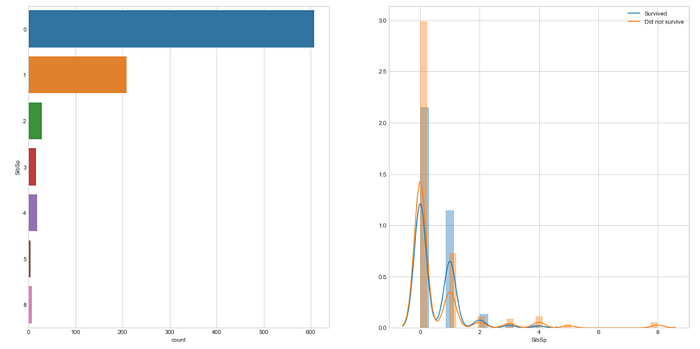
kde_kws={'bw': 0.2,"label": "Did not survive"});Feature: SibSp
Description: The number of siblings/spouses the passenger has aboard the Titanic.
How many missing values does SibSp has?
train.SibSp.isnull().sum()This line of code above returns 0. Let’s see number of unique values in this column and their distributions.
train.SibSp.value_counts()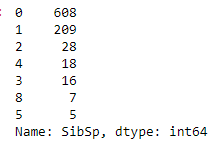
# Visualise the counts of SibSp and the distribution of SibSp #against Survivalplot_count_dist(train,label_column='Survived',target_column='SibSp', figsize=(20,10))
Let’s add SibSp feature to our new subset data frame.
#Add SibSp to new dataframe
df_new['SibSp'] = train['SibSp']
Feature: Parch
Description: The number of parents/children the passenger has aboard the Titanic.
Since this feature is similar to SibSp, we’ll do a similar analysis.
How many missing values does Parch has?
train.Parch.isnull().sum()This line of code above returns 0. Let’s see number of unique values in this column and their distributions.
train.SibSp.value_counts()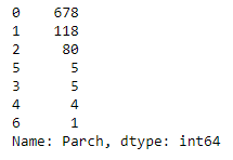
#Visualize the counts of Parch and distribution of values against #Survivalplot_count_dist(train,label_column='Survived',target_column='Parch',figsize=(20,10))

Feature: Ticket
Description: The ticket number of the boarding passenger.
How many missing values does Tickets have?
train.Ticket.isnull().sum()This line of code above returns 0. Let’s see number of unique values in this column .
train.Ticket.value_counts()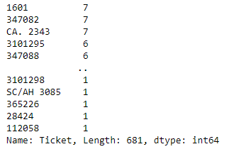
Here length of train.Ticket.value_counts() is 681 which is too many unique values for now. Let’s not include this feature in new subset data frame.
Feature: Fare
Description: How much the ticket cost.
How many missing values does Fare have? What kind of variable is Fare?
train.Fare.isnull().sum()
train.Fare.dtype
The code lines above returns 0 missing values and data type ‘float64’ . let’s see how many kinds of fare values are there?
train.Fare.value_counts()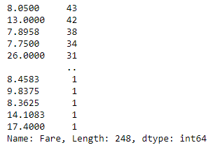
There are 248 different unique values in fare. Since fare is a numerical continious variable let’s add this feature to our new subset data frame.
df_new['Fare']= train['Fare']Feature: Cabin
Description: The cabin number where the passenger was staying.
How many missing values does Cabin have?
train.Cabin.isnull().sum()The code above returns 687.looks like there is 1/3 number of missing values in feature Cabin. So till we don’t have expert advice we do not fill the missing values, rather do not use it for the model right now. Let’s go to the next feature.
Feature: Embarked
Description: The port where the passenger boarded the Titanic.
Key: C = Cherbourg, Q = Queenstown, S = Southampton
How many missing values does Embarked have?
train.Embarked.isnull().sum()There are 2 missing values in Embarked column. Let’s see what kind of values are in Embarked.
train.Embarked.value_counts()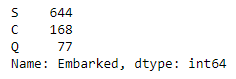
Looks like Embarked is a categorical variable and has three categorical options. Let’s count plot too.
sns.countplot(y='Embarked', data=train);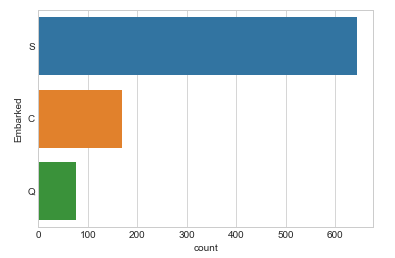
There are multiple ways to deal with missing values. Since only 2 values are missing out of 891 which is very less, let’s go with drooping those two rows with a missing value. But first, add this original column to our subset data frame.
# Add Embarked to new data frame
df_new['Embarked'] = train['Embarked']# Remove Embarked rows which are missing values
print(len(df_new))
df_new = df_new.dropna(subset=['Embarked'])
print(len(df_new))
The code block above will return 891 before removing rows and 889 after.
Feature Encoding:
Now we have filtered the features which we will use for training our model. But we still have a very important task to do. Feature encoding is the technique applied to features to convert it into numerical form(could be binary form or integer). It is very important to prepare the proper input dataset, compatible with the machine learning algorithm requirements. This will eventually improve the performance of machine learning models.
We can encode the features with one-hot encoding so they will be ready to be used with our machine learning models.
Let’s see original ‘df_new’ dataframe.
df_new.head()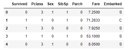
# One hot encode the categorical columns
df_embarked_one_hot = pd.get_dummies(df_new['Embarked'],
                                     prefix='embarked')df_sex_one_hot = pd.get_dummies(df_new['Sex'],
                                prefix='sex')df_plcass_one_hot = pd.get_dummies(df_new['Pclass'],
                                   prefix='pclass')
Now combine the one_hot columns with ‘df_new’.
# Combine the one hot encoded columns with df_con_enc
df_new_enc = pd.concat([df_new,
                        df_embarked_one_hot,
                        df_sex_one_hot,
                        df_plcass_one_hot], axis=1)# Drop the original categorical columns (because now they've been one hot encoded)
df_new_enc = df_new_enc.drop(['Pclass', 'Sex', 'Embarked'], axis=1)
Let’s look at ‘df_new_enc’ .
df_new_enc.head(10)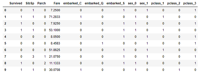
Start Building Machine Learning Models:
Now our data has been manipulating and converted to numbers, we can run a series of different machine learning algorithms over it to find which yield the best results.
Let’s select the data
# Seclect the dataframe we want to use for predictions
selected_df = df_new_enc
selected_df.head()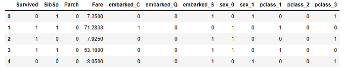
The first task to do with the selected data set is to split the data and labels.
# Split the dataframe into data and labels
X_train = selected_df.drop('Survived', axis=1) # data
y_train = selected_df.Survived # labels
Define a function to fit machine learning algorithms:
Since many of the algorithms we will use are from the sklearn library, they all take similar (practically the same) inputs and produce similar outputs. To prevent writing code multiple times, we will function fitting the model and returning the accuracy scores.
# Function that runs the requested algorithm and returns the accuracy metrics
def fit_ml_algo(algo, X_train, y_train, cv):

    # One Pass
    model = algo.fit(X_train, y_train)
    acc = round(model.score(X_train, y_train) * 100, 2)

    # Cross Validation
    train_pred = model_selection.cross_val_predict(algo,
                                                  X_train,
                                                  y_train,
                                                  cv=cv,
                                                  n_jobs = -1)
    # Cross-validation accuracy metric
    acc_cv = round(metrics.accuracy_score(y_train, train_pred) * 100, 2)

    return train_pred, acc, acc_cv
In the function above notice, we are obtaining both training accuracy and cross-validation accuracy as ‘acc’ and ‘acc_cv’. Cross-validation is a powerful preventative measure against overfitting. So we will consider cross-validation error while finalizing the algorithm for survival prediction.
Logistic Regression
# Logistic Regression
start_time = time.time()
train_pred_log, acc_log, acc_cv_log = fit_ml_algo(LogisticRegression(),
                                                               X_train,
                                                               y_train,
                                                                    10)
log_time = (time.time() - start_time)
print("Accuracy: %s" % acc_log)
print("Accuracy CV 10-Fold: %s" % acc_cv_log)
print("Running Time: %s" % datetime.timedelta(seconds=log_time))
Output:
Accuracy: 79.98
Accuracy CV 10-Fold: 79.42
Running Time: 0:00:43.517223
K-Nearest Neighbours
# k-Nearest Neighbours
start_time = time.time()
train_pred_knn, acc_knn, acc_cv_knn = fit_ml_algo(KNeighborsClassifier(),
                                                  X_train,
                                                  y_train,
                                                  10)
knn_time = (time.time() - start_time)
print("Accuracy: %s" % acc_knn)
print("Accuracy CV 10-Fold: %s" % acc_cv_knn)
print("Running Time: %s" % datetime.timedelta(seconds=knn_time))
Output:
Accuracy: 83.46
Accuracy CV 10-Fold: 76.72
Running Time: 0:00:02.552968
Gaussian Naive Bayes
# Gaussian Naive Bayes
start_time = time.time()
train_pred_gaussian, acc_gaussian, acc_cv_gaussian = fit_ml_algo(GaussianNB(),
                                                                      X_train,
                                                                      y_train,
                                                                           10)
gaussian_time = (time.time() - start_time)
print("Accuracy: %s" % acc_gaussian)
print("Accuracy CV 10-Fold: %s" % acc_cv_gaussian)
print("Running Time: %s" % datetime.timedelta(seconds=gaussian_time))
Output:
Accuracy: 78.52
Accuracy CV 10-Fold: 77.95
Running Time: 0:00:00.197989
Linear Support Vector Machines (SVC)
# Linear SVC
start_time = time.time()
train_pred_svc, acc_linear_svc, acc_cv_linear_svc = fit_ml_algo(LinearSVC(),
                                                                X_train,
                                                                y_train,
                                                                10)
linear_svc_time = (time.time() - start_time)
print("Accuracy: %s" % acc_linear_svc)
print("Accuracy CV 10-Fold: %s" % acc_cv_linear_svc)
print("Running Time: %s" % datetime.timedelta(seconds=linear_svc_time))
Output:
Accuracy: 75.93
Accuracy CV 10-Fold: 78.4
Running Time: 0:00:01.417908
Stochastic Gradient Descent
# Stochastic Gradient Descent
start_time = time.time()
train_pred_sgd, acc_sgd, acc_cv_sgd = fit_ml_algo(SGDClassifier(),
                                                  X_train,
                                                  y_train,
                                                  10)
sgd_time = (time.time() - start_time)
print("Accuracy: %s" % acc_sgd)
print("Accuracy CV 10-Fold: %s" % acc_cv_sgd)
print("Running Time: %s" % datetime.timedelta(seconds=sgd_time))
Output:
Accuracy: 78.18
Accuracy CV 10-Fold: 67.72
Running Time: 0:00:00.485966
Decision Tree Classifier
# Decision Tree Classifier
start_time = time.time()
train_pred_dt, acc_dt, acc_cv_dt = fit_ml_algo(tree.DecisionTreeClassifier(),
                                                                X_train,
                                                                y_train,
                                                                10)
dt_time = (time.time() - start_time)
print("Accuracy: %s" % acc_dt)
print("Accuracy CV 10-Fold: %s" % acc_cv_dt)
print("Running Time: %s" % datetime.timedelta(seconds=dt_time))
Output:
Accuracy: 92.46
Accuracy CV 10-Fold: 80.65
Running Time: 0:00:01.056698
Gradient Boost Trees
# Gradient Boosting Trees
start_time = time.time()
train_pred_gbt, acc_gbt, acc_cv_gbt = fit_ml_algo(GradientBoostingClassifier(),
                                                                       X_train,
                                                                       y_train,
                                                                       10)
gbt_time = (time.time() - start_time)
print("Accuracy: %s" % acc_gbt)
print("Accuracy CV 10-Fold: %s" % acc_cv_gbt)
print("Running Time: %s" % datetime.timedelta(seconds=gbt_time))
Output:
Accuracy: 86.61
Accuracy CV 10-Fold: 80.65
Running Time: 0:00:02.261205
CatBoost Algorithm
CatBoost is a state-of-the-art open-source gradient boosting on decision trees library. It’s simple and easy to use. And is now regularly one of my go-to algorithms for any kind of machine learning task.
For more on CatBoost and the methods it uses to deal with categorical variables, check out the CatBoost docs .
Anna Veronika Dorogush, lead of the team building CatBoost library suggest to not perform one hot encoding explicitly on categorical columns before using it because the algorithm will automatically perform the required encoding to categorical features by itself.
In my jupyter notebook of this blog post, I have used CatBoost for dataset before one hot encoding too. And you can see there the difference in accuracy. In this case, there was 0.22 difference in cross validation accuracy so I will go with the same encoded data frame which I used for earlier models for now.
# View the data for the CatBoost model
X_train.head()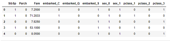
# View the labels for the CatBoost model
y_train.head()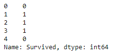
# Define the categorical features for the CatBoost model
cat_features = np.where(X_train.dtypes != np.float)[0]
cat_features
Output:
array([ 0, 1, 3, 4, 5, 6, 7, 8, 9, 10], dtype=int64)This means Catboost has picked up that all variables except Fare can be treated as categorical.
# Use the CatBoost Pool() function to pool together the training data and categorical feature labels
train_pool = Pool(X_train,
                  y_train,
                  cat_features)
Earlier we imported CatBoostClassifier, Pool, cv from catboost. Here Pool() function will pool together the training data and categorical feature labels. Now let’s fit CatBoostClassifier() algorithm in train_pool and plot the training graph as well.
# CatBoost model definition
catboost_model = CatBoostClassifier(iterations=1000,
                                    custom_loss=['Accuracy'],
                                    loss_function='Logloss')# Fit CatBoost model
catboost_model.fit(train_pool,
                   plot=True)# CatBoost accuracy
acc_catboost = round(catboost_model.score(X_train, y_train) * 100, 2)
This model took more than an hour to complete training in my jupyter notebook, but in google colaboratory only 53 sec. For cross-validation model trainning it took again more than an hour but in in google colaboratory only 6 min 18 sec.
Next , perform CatBoost cross-validation.
We performed crossviladation in each model above. So now let’s do for CatBoost too.
# How long will this take?
start_time = time.time()# Set params for cross-validation as same as initial model
cv_params = catboost_model.get_params()# Run the cross-validation for 10-folds (same as the other models)
cv_data = cv(train_pool,
             cv_params,
             fold_count=10,
             plot=True)# How long did it take?
catboost_time = (time.time() - start_time)# CatBoost CV results save into a dataframe (cv_data), let's withdraw the maximum accuracy score
acc_cv_catboost = round(np.max(cv_data['test-Accuracy-mean']) * 100, 2)
And then print out the CatBoost model metrics.
# Print out the CatBoost model metrics
print("---CatBoost Metrics---")
print("Accuracy: {}".format(acc_catboost))
print("Accuracy cross-validation 10-Fold: {}".format(acc_cv_catboost))
print("Running Time: {}".format(datetime.timedelta(seconds=catboost_time)))
Output:
---CatBoost Metrics---
Accuracy: 83.91
Accuracy cross-validation 10-Fold: 81.32
Running Time: 1:06:01.208055
Model Results:
Which model had the best cross-validation accuracy?
Note: We care most about cross-validation metrics because the metrics we get from .fit() can randomly score higher than usual.
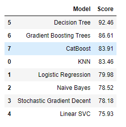
Regular accuracy scores
models = pd.DataFrame({
    'Model': ['KNN', 'Logistic Regression', 'Naive Bayes',
              'Stochastic Gradient Decent', 'Linear SVC',
              'Decision Tree', 'Gradient Boosting Trees',
              'CatBoost'],
    'Score': [
        acc_knn,
        acc_log,
        acc_gaussian,
        acc_sgd,
        acc_linear_svc,
        acc_dt,
        acc_gbt,
        acc_catboost
    ]})
print("---Reuglar Accuracy Scores---")
models.sort_values(by='Score', ascending=False)
Output:
Cross validation accuracy scores
cv_models = pd.DataFrame({
    'Model': ['KNN', 'Logistic Regression', 'Naive Bayes',
              'Stochastic Gradient Decent', 'Linear SVC',
              'Decision Tree', 'Gradient Boosting Trees',
              'CatBoost'],
    'Score': [
        acc_cv_knn,
        acc_cv_log,
        acc_cv_gaussian,
        acc_cv_sgd,
        acc_cv_linear_svc,
        acc_cv_dt,
        acc_cv_gbt,
        acc_cv_catboost
    ]})
print('---Cross-validation Accuracy Scores---')
cv_models.sort_values(by='Score', ascending=False)
Output:
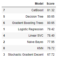
We can see from the tables, the CatBoost model had the best results. Getting just under 82% is pretty good considering guessing would result in about 50% accuracy (0 or 1).
We’ll pay more attention to the cross-validation figure.
Cross-validation is more robust than just the .fit() models as it does multiple passes over the data instead of one.
Because the CatBoost model got the best results, we’ll use it for the next steps.
Submission
So we are using CatBoost model to make a prediction on the test dataset and then submit our predictions to Kaggle.
We have same kind of columns for test data set in which our model is trained on.
So we have to select the subset of same columns of the test dateframe, encode them and make a prediciton with our model.
# We need our test dataframe to look like this one
X_train.head()# Our test dataframe has some columns our model hasn't been trained on
test.head()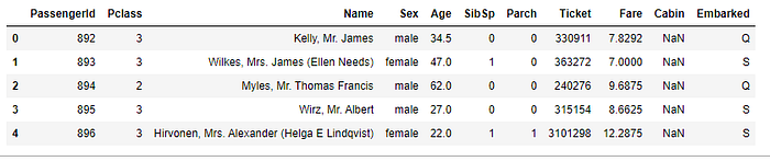
Let’s do One hot encoding in respective features.
test_embarked_one_hot = pd.get_dummies(test['Embarked'],
                                       prefix='embarked')test_sex_one_hot = pd.get_dummies(test['Sex'],
                                prefix='sex')test_plcass_one_hot = pd.get_dummies(test['Pclass'],
                                   prefix='pclass')
Then combine the test one hot encoded columns with test.
test = pd.concat([test,
test_embarked_one_hot,
test_sex_one_hot,
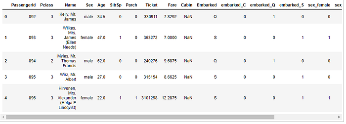
test_plcass_one_hot], axis=1)# Let's look at test, it should have one hot encoded columns now
test.head()
Before making a prediction using the CatBoost model let’s check the columns names are either same or not in both test and train set. We did one hot coding in some columns so that will create new column name.
test.columnsOutput:
Index(['PassengerId', 'Pclass', 'Name', 'Sex', 'Age', 'SibSp', 'Parch','Ticket', 'Fare', 'Cabin', 'Embarked', 'embarked_C', 'embarked_Q','embarked_S', 'sex_female', 'sex_male', 'pclass_1', 'pclass_2','pclass_3'],dtype='object')Columns in X_train:
X_train.columnsOutput:
Index(['SibSp', 'Parch', 'Fare', 'embarked_C', 'embarked_Q', 'embarked_S','sex_0', 'sex_1', 'pclass_1', 'pclass_2', 'pclass_3'],
 dtype='object')
You can see the new column names for sex column’s dummies are different. let’s rename ‘test.columns’ name.
test.rename(columns={"sex_female": "sex_0", "sex_male": "sex_1"},inplace=True)Now let’s select the columns which were used for model training for predictions.
# Create a list of columns to be used for the predictions
wanted_test_columns = X_train.columns
wanted_test_columns
Output:
Index(['SibSp', 'Parch', 'Fare', 'embarked_C', 'embarked_Q', 'embarked_S','sex_0', 'sex_1', 'pclass_1', 'pclass_2', 'pclass_3'],
dtype='object')
Make a prediction using the CatBoost model on the wanted columns.
predictions = catboost_model.predict(test[wanted_test_columns])# Our predictions array is comprised of 0's and 1's (Survived or Did Not Survive)
predictions[:20]
Output:
array([0, 0, 0, 0, 1, 0, 1, 0, 1, 0, 0, 0, 1, 0, 1, 1, 0, 0, 0, 1])Now create a submission data frame and append the predictions on it. Remember we already have sample data frame for how our submission data frame must look like. First let’s create submission data frame and then edit.
# Create a submisison dataframe and append the relevant columns
submission = pd.DataFrame()
submission['PassengerId'] = test['PassengerId']
submission['Survived'] = predictions # our model predictions on the test dataset
submission.head()
# What does our submission have to look like?
gender_submission.head()if len(submission) == len(test):
print("Submission dataframe is the same length as test ({} rows).".format(len(submission)))
else:
print("Dataframes mismatched, won't be able to submit to Kaggle.")Output:
Submission dataframe is the same length as test (418 rows).Convert submisison dataframe to csv for submission to csv for Kaggle submisison.
submission.to_csv('../catboost_submission.csv', index=False)
print('Submission CSV is ready!')
Output:
Submission CSV is ready!You must have already signed in in Kaggle.com .So for submission go to the page of Titanic: Machine Learning from Disaster and got to My Submissions tab.

Click on submit prediction and upload the submission.csv file and write a few words about your submission.
Wait for a few seconds, you will see the Public Score of your prediction.
Congratulations! You did it.
Keep learning feature engineering, feature importance, hyperparameter tuning, and other techniques to predict these models more accurate.
Learn More
Sklearn Classification Notebook by Daniel Furasso
Encoding categorical features in Python blog post by Practical Python Business
CatBoost Python tutorial on GitHub
References
Hands-on Exploratory Data Analysis using Python, By Suresh Kumar Mukhiya, Usman Ahmed, 2020, PACKT Publication
“Your-first-kaggle-submission” by Daniel Bourke
Thanks for being with this blog post. I suggest you have a look at my jupyter notebook in this github repository. Here I have done some more work for feature importance analysis.
If you are a beginner in the field of Machine Learning a few things above might not make sense right now but will make as you keep on learning further.
Keep Learning
asha.gaire95@gmail.com

